Weather: Going Into the Upper Air

Going Into the Upper Air

The ground-level data nicely shows what's occurring outside your window or outside the window of a weather station a thousand miles away. Sometimes that's enough to make a forecast for the next few days, but usually, we need to dig deeper—or, in this case, go to a higher level. In "Measuring the Atmosphere," we looked at radiosonde balloons that are launched twice daily around the world. The data these balloons provide is invaluable. From that information, maps representing different levels of atmospheric conditions are put together. These show the true multidimensional character of the atmosphere.

One of my favorite maps is called the 500-millibar (mb) map, which shows the flow of the atmosphere at a level where the pressure is about half the pressure of the surface. On these constant pressure charts, the pressure is the same in New York as it is in Los Angeles, but the elevation at which that pressure is found is different. Contours that show the elevation of the surface are drawn. The following figure shows the 500-mb chart that I used in the weather office. On the upper-air charts, contours are drawn every 60 meters. A contour labeled 576 means that the 500-mb surface is 5,760 meters above the ground.

The notations "L" and "H" indicate locations of low and high elevation of the pressure surface. The dashed lines indicate the temperature in degrees C. Those lines of constant temperature are called isotherms. The station locations are represented, with the temperature reading in the upper left of the data array, the dew point-temperature difference in the lower left, the elevation in the upper right (add a zero for height in meters), and the standard wind barbs indicating wind direction and speed.

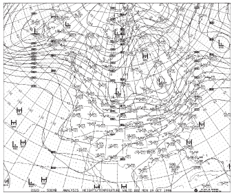
500-millibar map, October 19, 1998.

But let's not get lost in all this symbolism. What I was looking for on this map this Monday morning was the general flow of the atmosphere. The 500-mb chart is great for that. It shows the general direction of weather. Although the jet stream itself is located at a much higher level, above 10 kilometers, the flow at around five kilometers is indicative of the way weather systems are moving. Notice how the flow is generally along those contours. In this case, the weather that was heading for Connecticut originated in southern Illinois and southern Indiana. Also the flow was generally from west to east, but there was a big "High" anchored off the southeast coast.

This told me a lot. First the front moving through eastern New York and New England had some pretty good push behind it. The west-to-east flow would move it along, which seemed to agree with the satellite and Doppler pictures. Also the flow was not from the north, so any change toward cooler weather would probably be gradual. If that flow had been sweeping down from central Canada, the temperature would have dropped sharply, but in this case, the weather was more moderate immediately behind the front.

The flow at 500 mb usually represents the average flow in the atmosphere, and surface weather systems move at an average of half the speed at this level. The wind flow between New England and the Midwest is about 60 knots. So surface weather will move along at a rate of 60 divided by 2, or 30 knots. Now, if the pattern is changing slowly, and it often is, then the air is pushing along at 30 knots and over a 24-hour period the air will cover a distance of 720 miles (30 times 24).

If I want to see what type of air mass is arriving, I will go back from the air stream to a position 720 miles away. That would place me in southern Illinois. The air mass arriving on this day was over southern Illinois about 24 hours ago. This is far from exact and loaded with problems, but as a first and often best estimate of conditions for the upcoming day, it works. So what was it like yesterday in southern Illinois?

The first figure below shows the high temperatures for the previous day, Sunday, across the entire country. I saw that in southern Illinois, the temperature reached the upper 60s, close to 70 degrees. I know that I'll be predicting a high temperature close to that. But to get a second opinion of the high temperature, I looked at another upper-level chart.

This one is at the 850-mb level. This 850-mb chart is useful in many ways (see the second figure below). The coding and format are exactly the same as the 500-mb chart, but this chart shows a pressure surface that is closer to the ground, usually about 1,500 meters. This chart is useful for predicting precipitation. Normally precipitation occurs when the temperature-dew point difference is 5 degrees or less. The smaller the difference, the closer that layer is to saturation. At 5 degrees or less, the difference is small enough to support condensation at a level that's frequently near the base of clouds. I quickly saw that the difference was large overhead, but upwind, in southwest Pennsylvania, the difference was just 1 degree. This chart was prepared from data taken at 8 P.M.on Sunday. Evidently the showers that raced into the region overnight came from that region of moist air in western Pennsylvania, just 12 hours earlier. Now, for that particular Monday morning, I used this data to help determine the upcoming day's high temperature.

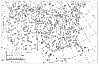
High temperatures observed for October 19, 1998.

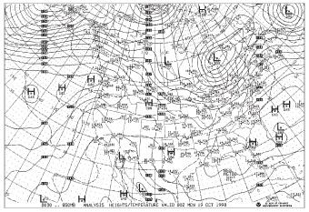
850-millibar for October 19, 1998.

I have a trick. If the atmosphere is stirred up and if there's maximum sunshine without any strong air mass being blown into the region, I'll add 28 degrees F to the 850-mb temperature to arrive at the day's maximum. In this case, the trajectory of air is coming from southern Illinois, where the 850-mb temperature is 10 degrees C, which converts to 50 degrees F. If I add 28 degrees to that, the temperature becomes 78 degrees, which would be the absolute highest the temperature could go. The 28-degree figure comes from the temperature change that a bundle of air would undergo if it sank from about 5,000 feet to the surface. The rate of warming, called the adiabatic lapse rate, comes to 5.5 degrees for every thousand feet. (I rounded up from 27.5 to 28 degrees.) It's not an exact technique. On that day, the 850-mb surface was at 1,500 meters, less than 5,000 feet above the ground. But for a quick, upper limit for the temperature, the technique works. So the surface maps suggest a high near 70, and this chart suggested the upper 70s. I took an average and put in a high temperature forecast for the mid-70s.

At this point, I felt confident enough to go on the air. All indicators pointed to a day without rain and a temperature in the 70s. The skies will probably have some cloudiness, but plenty of sunshine was expected. Colder weather will eventually develop, but it will arrive slowly during the day. But of course, perfection is the aim, and we could do some fine-tuning. Let's check out the assortment of computer information that's readily available.

Excerpted from The Complete Idiot's Guide to Weather © 2002 by Mel Goldstein, Ph.D.. All rights reserved including the right of reproduction in whole or in part in any form. Used by arrangement with Alpha Books, a member of Penguin Group (USA) Inc.