Look at These Prices!: Tinkering with Markets
Tinkering with Markets
Up to now we have been examining the way markets operate when they are left to their own devices. However, markets are rarely left to their own devices. External measures are often introduced into a market, often by the government, sometimes by business. These interventions can affect the price of a product or service, the quantity demanded, and the behavior of producers and consumers. The rest of this section examines some of these measures—specifically, sales taxes, rent controls, and the minimum wage—and their effect on supply and demand.
Please note that I intend only to show the effects of these measures on the market purely from the economic standpoint. I am neither addressing nor judging the social impact or political aspects of these measures.
A Sales Tax Is a Price Increase
EconoTalk
Interventions in the market consist of steps by the government (price controls), businesses (monopolies), or even consumers (boycotts or trade unions) that affect the price, quantity, demand, supply, or some other aspect of the market. In general, however, the term market intervention refers to government actions. The parties doing the intervening generally believe that they are doing so for a good reason.
A price ceiling is a government-mandated maximum price that a seller can charge for a product or service. A price floor is a government-mandated minimum price that a seller can charge. Rent control is an example of a price ceiling, while a minimum wage is in effect a floor on the price of labor.
The poverty threshold (sometimes called “the poverty line”) is the level of annual household income, adjusted for household size, which officially defines poverty. A household that earns an income below the threshold is “officially” poor, and eligible for certain types of public assistance. The U.S. Census Bureau updates these data every year to reflect changes in incomes and price levels.
Sales taxes are levied by all states (except New Hampshire) and many cities as a way of raising revenue. Each individual state or city decides the amount of sales tax to charge, usually a small percentage—around or less than 5 percent—of the purchase price.
The term “sales tax” refers to a general tax on purchases. In some jurisdictions certain items, such as food or clothing, are exempt from sales tax. Also, the term “sales tax” does not usually apply to taxes on specific goods. For instance, taxes on gasoline and so-called “sin taxes” on cigarettes and alcoholic beverages are called gasoline and cigarette taxes and so on. Despite their titles, they are a form of sales tax and have the same general effect.
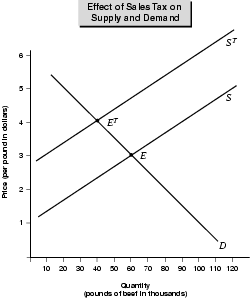
That effect is to increase the price of the item being purchased. As you know by now, the law of supply and demand dictates that if the price increases, the -quantity demanded decreases. As Figure 5.6 shows, that is exactly what happens when a sales tax is levied.
Here we return to our Supply, Demand, and the Invisible Hand example of the market for beef. Figure 5.6 shows that the equilibrium price without the sales tax is $3 a pound. At that price, consumers demand 60,000 pounds of beef. The chart assumes a sales tax of $1 per pound of beef (don't laugh, cigarette taxes are often well over $1 a pack). The tax raises the price, but notice that overall demand for beef—the demand curve—does not shift. Instead, demand decreases along the existing demand curve to 40,000 pounds.
The price increase does, however, shift the supply curve. The shift reflects the new reality imposed by the “higher price” under the sales tax. Supply curve ST in the chart shows that, given the decreased demand due to the higher price, suppliers are willing to supply less beef at all price levels. Therefore, the new equilibrium point (ET) stands at a price of $4 (equal to $3 plus the $1 tax) and a quantity of 40,000 pounds.
As a result of the tax, the producers supply and consumers demand 20,000 fewer pounds of beef. In effect, the tax on beef takes 20,000 pounds of beef off the market. These dynamics hold true for most sales taxes on most products. There are arguments for and against sales taxes and “sin taxes,” but without question, they alter the prices and quantities that would prevail in the market if they were absent. However, they do raise tax revenues.
Rent Controls
Some communities employ rent controls to make affordable housing available to people without enough income to otherwise live in the community. In general, rent controls keep the price of rental units below the market price. Indeed, that is their goal, because at the market price there's not enough housing for people with lower incomes.
If you consider the relationship between price and quantity in a free market, you'll realize that over time the effect of rent control will be to limit the amount of housing available in the community. Why? Because if the price ceiling is below the market price (that is, the price at the equilibrium point), then the quantity of housing will be kept below the point that buyers would demand in a free market. Figure 5.7 illustrates this.
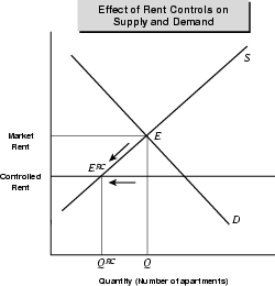
The price ceiling imposed by rent control creates a shortage of housing and leads to some renters being unable to find apartments. In Figure 5.7, the shortage is the difference between the “imposed equilibrium quantity” of QRC and the market equilibrium quantity of Q.
In practice, rent controls do limit construction of new rental units in the long run, as has been seen in New York and other cities. New Yorkers lucky enough to live in rent-controlled apartments love the system. But, over time, landlords found that the costs of buying or constructing and maintaining a building outpaced the rent increases permitted under the controls. That made owning an apartment building a bad business proposition and led landlords to abandon buildings. A two-tier system developed, in which people with rent-controlled apartments paid rents well below market rates and those in decontrolled apartments or new buildings not subject to rent control had to pay market-rate rents well above what they would have been in a free market.
Again, the social value of making affordable housing available to lower income people is left out of this analysis. Yet the danger in rent controls (as opposed to other means of helping people afford housing, such as welfare payments to raise their incomes) is that a city can wind up with two levels of housing—very inexpensive and very expensive. This tends to squeeze middle income people out of the city. This also occurred to an extent in New York, although other factors ranging from decaying schools to rising crime also played a role in the movement of middle class people out of the city.
The Minimum Wage
While rent control sets a ceiling on the cost of housing, the minimum wage sets a floor under the price of labor. Minimum wage legislation aims to provide every worker with a “living wage,” meaning an hourly rate that covers the cost of life's necessities.
Whether the current minimum wage does that is open to debate. Working a 40-hour week, at the current U.S. minimum wage of $5.15, a worker would earn $206 a week, or about $10,700 a year. According to the U.S. Census Bureau, the poverty threshold for one person is currently a little over $9,000 a year. For a household of two people the threshold is $11,600. Therefore, the minimum wage keeps a single person just above the official definition of poverty. It fails to do the same for a household of two with one breadwinner, let alone a household with one or more children and a full-time homemaker.
All of this aside, an economist would analyze the effect of a minimum wage on the labor market as depicted in Figure 5.8.
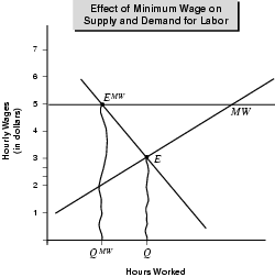
If the minimum wage is set above the wage that would otherwise prevail in the free market, then the wage floor will generate unemployment. Figure 5.8 shows why.
The line labeled MW at the $5.00 wage level represents the minimum wage, while the free market wage stands at $3.00. The minimum wage creates an “imposed equilibrium point” (EMW) at which the quantity of labor demanded (QMW) stands well below the quantity that employers would demand (Q) at the free market wage of $3.00. This generates a surplus of labor (that is, idle workers) equal to Q minus QMW. Workers who are lucky (or skilled) enough to land a job at the minimum wage are happy. However, many of those who cannot command the minimum wage are unemployed.
The Wages of Control
Thus in the case of rent control and the minimum wage, government intervention in free markets distorts the dynamics of supply and demand. In the case of rent control, a city winds up with too little housing, or with a two-tier system. In the two-tier system, some lucky people enjoy apartments at below-market rates, while others are paying inflated rates for a scarcer number of “free market” apartments.
In the case of the minimum wage, some workers are idle because the government is, in effect requiring them to demand a wage that employers are not willing to pay. This may have the unintended consequence of actually putting less money into the workers' pockets.
There are good arguments for and against rent control and the minimum wage. Here, however, the goal is to examine their “pure” effect on supply and demand. To do this, we are leaving social aims and other factors, such as welfare payments and differences in the cost of living around the nation, out of the discussion for the moment.
Excerpted from The Complete Idiot's Guide to Economics © 2003 by Tom Gorman. All rights reserved including the right of reproduction in whole or in part in any form. Used by arrangement with Alpha Books, a member of Penguin Group (USA) Inc.
To order this book direct from the publisher, visit the Penguin USA website or call 1-800-253-6476. You can also purchase this book at Amazon.com and Barnes & Noble.
Trending
Here are the facts and trivia that people are buzzing about.